Appendix B
Computing Boundary Layer Value Correction
The development of boundary layers along supersonic intake surfaces presents a significant aerodynamic challenge that directly influences the external compression shock structure. When high-speed air flows along intake surfaces, it does not simply follow the geometric contours we design on paper. Instead, it creates a thin layer of affected flow—the boundary layer—that effectively reshapes the path air takes through the intake. This appendix explores how we account for these boundary layer effects through what is called the Boundary Layer Value Correction (BLVC).
B.1 Displacement Thickness
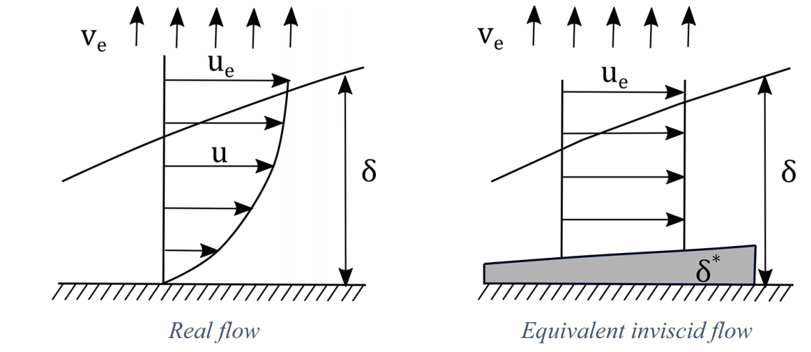
In an ideal world, air would follow the surface of the external compression ramps. However, the reality is more complex—the boundary layer causes the main flow to deviate from this intended path. To quantify this deviation, we use the concept called displacement thickness, denoted by δ*.
As shown in Figure B.1, displacement thickness represents how much the boundary layer "pushes" the main flow away from the wall. Mathematically, we express this as:
where δ is the boundary layer thickness, and y represents the wall-normal distance. Equation (B.1) integrates the flow properties through the boundary layer, giving us a measure of its effective thickness.
B.2 Methodology for Boundary Layer Analysis
The implementation of boundary layer analysis relies on systematic computational fluid dynamics (CFD) data processing. The methodology employs wall-normal probe lines oriented perpendicular to the ramp surface, as depicted in Figure B.2. These probe lines serve as discrete sampling locations for flow property extraction, establishing the foundation for boundary layer characterization and subsequent geometric corrections.

B.3 Boundary Layer Edge Detection
The boundary layer edge, defined by δ, is critical for calculating δ* accurately. In flows without significant pressure gradients, this edge is typically defined as the point where the wall-normal velocity reaches 99% of the freestream velocity, Ue, as shown in Figure B.1.
However, in cases with strong pressure gradients, such as those encountered in intakes, defining a stable Ue value is challenging. An initial estimate for the boundary layer edge can instead be obtained using a vorticity-based criterion [1]:
Where CΩ is an empirical parameter taken as 0.02 for the standard boundary layer thickness criterion of 99% of freestream velocity [1]. This criterion identifies the boundary layer edge based on the wall-normal vorticity threshold, capturing boundary layer behavior up to a certain limit, as illustrated in Figure B.3 for E3 theoretical supersonic intake. The boundary layer thickness obtained is shown using the white line over the contours of z-vorticity in Figure B.3.
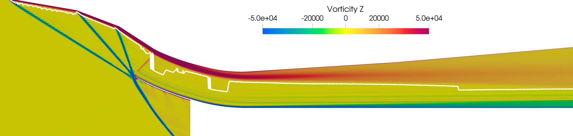
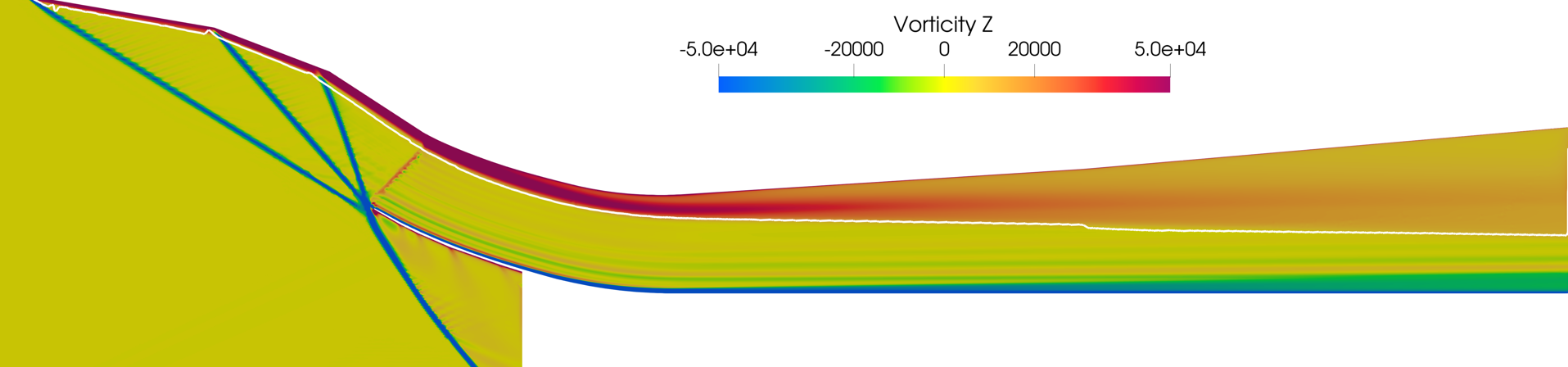
Near high-vorticity regions, such as downstream of terminal shocks, the vorticity-based approach can lose accuracy. A sudden jump in the white line in Figure B.3 behind the terminal shock illustrates the difficulty this method faces in high-vorticity regions. To address this, a secondary filter using the local velocity profile is applied on top of the first vorticity-based filter, refining the boundary layer edge:
This combined approach, illustrated in Figure B.4, offers a more precise measurement of the boundary layer, particularly in complex flow regions.
B.4 Displacement Thickness and Ramp Angle Corrections
The calculated displacement thickness distribution, visualized in Figure B.5 by the white line, exhibits characteristic streamwise growth with distinct discontinuities across shock waves. The angular difference between the displacement thickness distribution and the original ramp geometry determines the requisite corrections to the ramp angles. These corrections ensure that the effective flow path, incorporating boundary layer effects, generates shock structures consistent with the theoretical design specifications.
This approach to boundary layer correction maintains broad applicability across external and mixed compression intake configurations. The methodology establishes a framework for reconciling theoretical design parameters with viscous flow effects, ultimately closing the gap between the theoretically expected aerodynamic performance and that practically obtained in real-world applications for supersonic intakes.

References
- Uzun, A., and Malik, M. R., "Simulation of a Turbulent Flow Subjected to Favorable and Adverse Pressure Gradients," Theoretical and Computational Fluid Dynamics, Vol. 35, No. 3, 2021, pp. 293–329. https://doi.org/10.1007/s00162-020-00558-4